Summary

Agent capabilities abstract behaviors and abilities that are recurrent in agents.

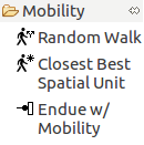
Mobility

The mobility capability gives the agent the ability to move.

Fig. 1 shows all the objects related to the mobility capability that can be managed on the ABStractme Tool.

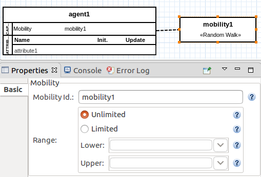
The random walk mobility provides randomized movement to the agent. The range can be either unlimited or limited by a specific value.

In the case of a limited range, attributes of the type INTEGER can be used as the upper or lower bounds.

Fig. 2. shows the box that represents the random walk mobility on the diagram along with the properties view to edit the mobility id and its range.

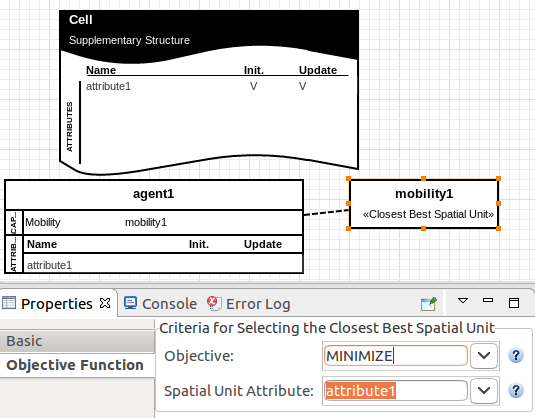
The closest best mobility uses a criterion to define the best position for the agent to move towards to.

Fig. 3 shows the box that represents the closest best mobility on the diagram along with the properties view to edit the mobility id and its range.

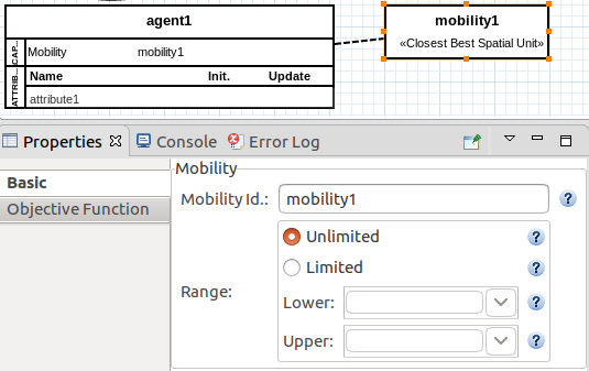
The closest best mobility needs a supplementary structure attribute to be the criteria for the best position to move to, either the place where the attribute value is the smallest or biggest from all available locations.

Fig. 4 shows the properties view where the attribute can be set, with the objective being to minimize (smallest value) or to maximize (highest value).

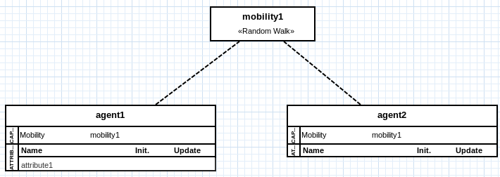
The mobility capabilities can be shared between more than one agent to avoid having to set the same mobility for every agent, as shown in Fig. 5.

Surviving

The surviving capability represents conditions for an agent to die. An agent death can happen by age (after a defined number of timesteps) or by depletion of energy(example: starvation) or even a custom condition.

Fig. 6 shows all the objects related to the surviving capability that can be managed on the ABStractme Tool.

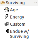
Fig. 7 shows the box that represents the living age capability on the diagram along with the properties view to edit the living id.

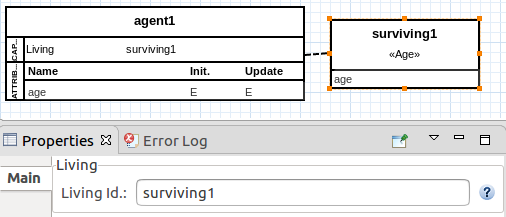
Fig. 8 shows the properties view to edit the age attribute.

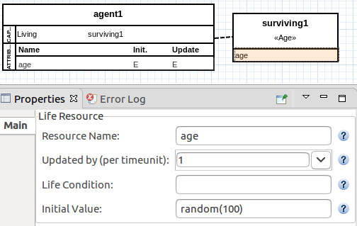
Fig.9 shows the properties view to edit the energy attribute.

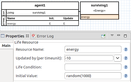
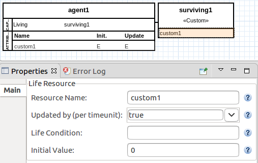
Fig.10 shows the properties view to edit the custom attribute.

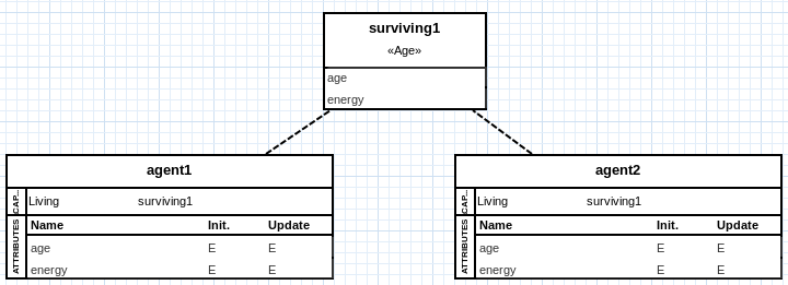
The surviving capabilities can be shared between more than one agent to avoid having to set the same for every agent, as shown in Fig. 11.

Decision Capabilities

A decision capability represents a decision policy for selecting one option from all the available decision options.

To use a decision capability, an agent must have a decision capability set as update source of an attribute.

Decision capabilities represent decision policies for updating attributes. When an attribute specifies a decision capability as the update source, the decision capability decides (selects) the attribute value at each timestep.

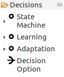
Fig. 12 shows all the objects related to the decision capabilities that can be managed on the ABStractme Tool.

Any decision capability has a decide() operation, to determine what decision option must be selected given its decision policy.

The set of available decision options can be static, or dynamic.

Static decision options are specified by the designer during the model specification.

What can be static options: Actuators, actuator groups, actuator states, or activations (flow control capability).

Other decision capabilities can also be set as static options. In that case, the output of the decision capability is considered as a decision option.

If the set of static options is homogeneous (i.e., has many actuator states (flow control capability) or has many decision capabilities), each particular element/value is considered as a decision option.

In turn, if the set of static options is heterogeneous (i.e., has actuators and actuator states, or has actuator states and actuator groups (flow control capability)), the cartesian product between the different elements is considered as decision options.

Dynamic decision options exist only during the execution of the simulation. We assume that these dynamic values are stored in an agent attribute (i.e., a perception attribute, which is updated at each timestep with the entities the perceived by the agent).

By definition, the set of dynamic options is always homogeneous. Therefore, previous notes on heterogeneous options are not applied for dynamic options.

The type of the attribute whose update source is a decision capability must be consistent with the decision options of the capability (either static or dynamic).

Connections (arrows) are used to represent which elements of the model are decision options of a decision capability.

Three types of decision capabilities are supported: state machines, learning, and adaptation. They are described in the following sections.

State machine

A state machine capability represents a fixed decision policy.

A state machine is represented by a box with the following two sections:

i) the state machine identification: any valid string (spaces are allowed).

ii) its transitions(each transition has an option, condition and a target state).

The decision options list is only visible in the properties view.

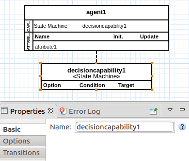
Fig. 13 shows the box that represents the state machine on the diagram along with the properties view to edit the state machine id.

A state machine is composed of states and transitions.

Each state represents a decision option.

The selected option of a state machine is its current state.

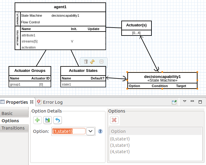
Fig. 14 shows the properties view to edit the state machine decision options list.

A state transition is described by a transition expression (that specifies the condition that triggers the transition) and a target state.

The transition condition can be:

i) a temporal value: the transition is triggered when the temporal value is reached.

ii) a boolean expression: the transition is triggered when the expression is evaluated to true.

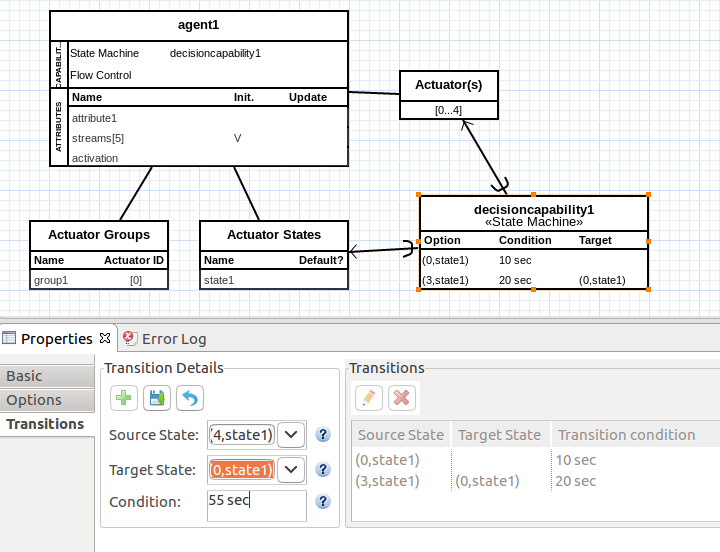
Fig. 15 shows the properties view to edit the state machine transitions.

Learning

A learning capability abstracts a learning technique to allow an agent to learn a decision policy.

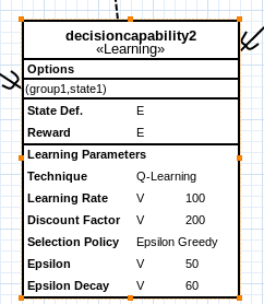
A learning capability is represented by a box with the following five sections:

i) the learning capability identification: any valid string (spaces are allowed).

ii) its decision options.

iii) its states (state definition).

iv) the reward definition.

v) the learning technique and its learning parameters.

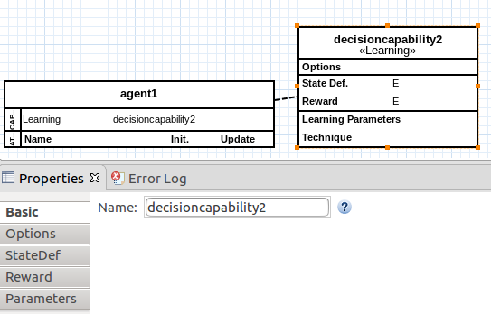
Fig. 16 shows the box that represents the learning capability on the diagram along with the properties view to edit the learning capability id.

The actions of a reinforcement learning are the decision options provided as input for the capability. The selected action is available as the decision output.

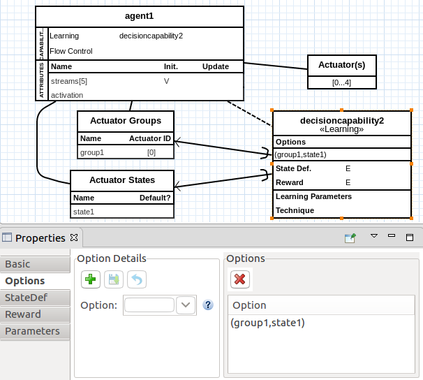
Fig. 17 shows the properties view to edit the learning capability decision options list.

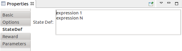
States of a reinforcement learning capability are a tuple that describes all the parts that compose a state as expressions. The actual states are created during the simulation, from the combination of expression values.

Fig. 18 shows the properties view to edit the learning capability states.

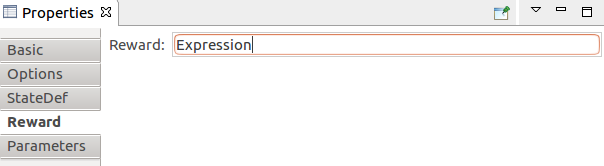
The reward of a reinforcement learning capability is specified as an expression, which can consider any model element.

Fig. 19 shows the properties view to edit the learning capability reward.

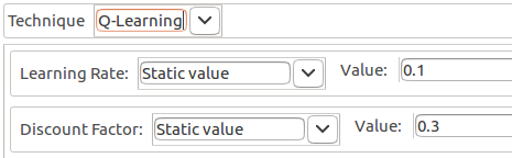
A learning technique usually has learning parameters, which guide the learning process. These parameters are represented as attributes of the learning technique, to which sources can be associated to provide parameter values, as shown in Fig. 20.

The technique is of the type reinforcement learning, with which agents learn through experience. As agents act on the environment, they receive a reward signal based on the outcomes of previous states and actions. The reinforcement learning capability provided in our model is the Q-Learning technique.

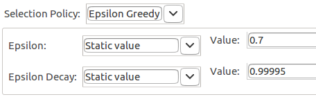
Both Fig. 21 and Fig. 22 demonstrate how to edit the learning parameters in the properties view.

Adaptation

An adaptation capability represents an adaptive decision policy.

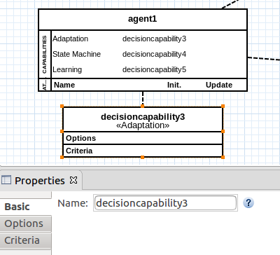
An adaptation is represented by a box with the following three sections:

i) the adaptation identification: any valid string (spaces are allowed).

ii) its decision options.

iii) the criterion.

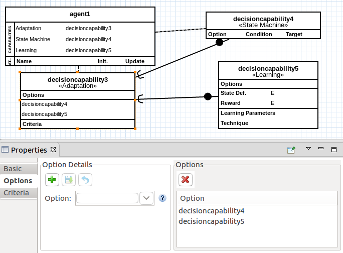
Fig. 23 shows the box that represents the adaptation capability on the diagram along with the properties view to edit the adaptation id.

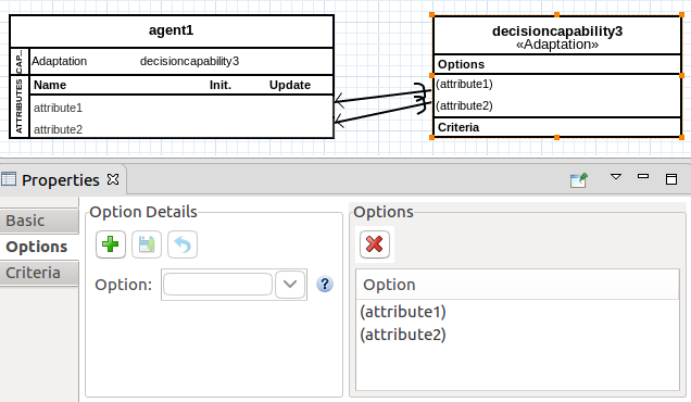
As with any other decision capability, the adaptation capability can have static (Fig. 24) or dynamic(Fig. 25) options, set by making relationships of the type Decision Option to other elements of the model, via the Decision Option row on the palette.

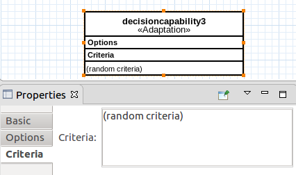
The adaptive decision policy is represented by an adaptation criterion.

The adaptation criterion is specified by an expression that describes which option should be selected among the decision options available — the one that meets the criterion.

Fig. 26 shows the properties view to edit the adaptation criterion.

Flow Control

A flow control capability represents the ability to regulate the flow of a set of streams using its actuators.

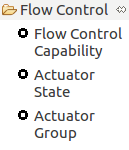
Fig. 27 shows all the objects related to the flow control capability that can be managed on the ABStractme Tool.

A flow control capability implies that the agent has a set of streams. These are represented as a streams attribute in the agent. The number of streams is specified by the cardinality of this attribute.

A flow control capability also implies that the agent has an additional attribute to specify the activation that is selected at the current timestep.

A flow control capability is represented as by the literal ’Flow Control’, which is shown in the capability section of the agent box, as seen in Fig. 28, along with the streams and activation attributes.

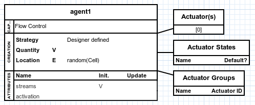
To regulate flow, it is assumed that the agent has a set of regulators and that these regulators can be in certain states.

Regulators can be seen as actuators of the agent, which are identified by a number. Such identifier relates the actuator to the corresponding stream it is regulating (i.e., a regulator 0 is in charge of regulating the stream 0, and so on). Actuators can be grouped into actuator groups, on which all activate the same state simultaneously. Consequently, a group is considered a single actuator because both are considered actuatable devices. Actuatable devices are considered mutually exclusive: only one actuator or group can assume a non-default state at a given moment; all others remain in the default state.

For the actuators element, its bottom section shows the identifiers of the actuators. These identifiers are generated automatically, according to the cardinality of the streams attribute. The user can not change these identifiers. They are shown just to allow further connections from decision capabilities.

Notice that:

i) The number of identifiers matches the cardinality of the "streams" attribute of the agent (described previously).

ii) There is a correspondence between the identifiers and the stream it manages: the actuator 0 is in charge of regulating the stream 0, and so on.

For the actuator states element, its bottom section presents all the specified actuator states, one per row. Each row shows the state name and a symbol that indicates whether it is a default state. They can be edited on the properties view as shown in Fig. 29.

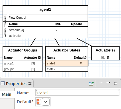
The actuator state that is automatically activated when no other state is active is the default state.

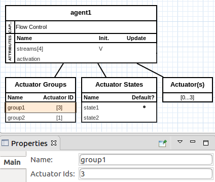
For the actuator groups element, its bottom section presents all the specified actuator groups, one per row. Each row shows the group name and the identifiers of its related actuators and can be edited on the properties view, as shown in Fig. 30.

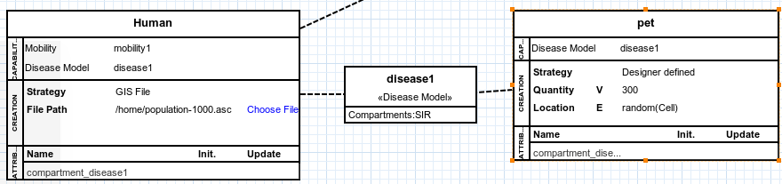
Diseases

The disease capability gives the agent the ability to be affected by a disease.

Fig. 31 shows all the objects related to the disease capability that can be managed on the ABStractme Tool.

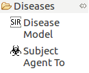
Fig. 32 shows the box that represents the disease capability on the diagram.

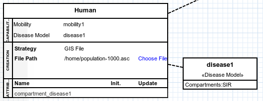
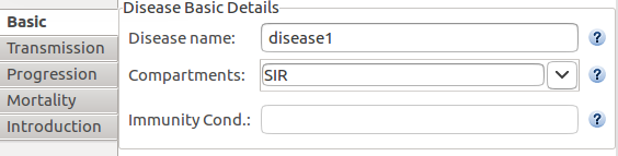
When first setting a disease, its identification and compartments must be specified on the basic properties tab.

Fig. 33 shows the box that represents the properties view to edit the disease basic details.

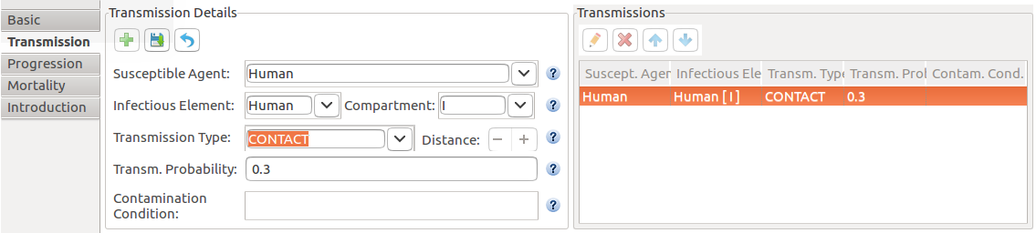
The transmission tab on the properties view specifies a contamination interaction:

Susceptible Agent: the agent that will be contaminated.

Infectious Element: agent or entity that transmits the disease.

Compartment: infectious compartment.

Transmission Type: can be by contact or proximity.

Transmission Probability: the probability of transmission (between 0.0 and 1.0).

Contamination Condition: to use when there is a restriction in the contamination.

Fig. 34 shows the box that represents the properties view to edit the disease transmission.

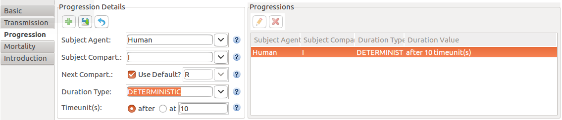
The progression tab on the properties view specifies the duration of a compartment:

Subject Agent: the agent subjected to the duration.

Subject Compartment: the compartment subjected to the duration.

Next Compartment: next compartment to transition to, after the duration.

Duration Type: the type of duration, can be:

i) Deterministic: when the duration is a fixed value.

ii) Probabilistic: the probability of recovery.

iii) Conditional: duration end on a certain condition.

iv) Custom: a combination of the above.

Fig. 35 shows the box that represents the properties view to edit the disease progression.

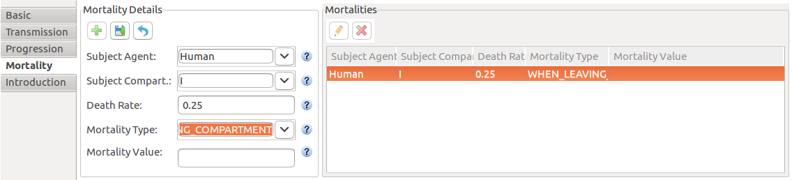
The mortality tab on the properties view specifies a death rate for the infected agents:

Subject Agent: the agent that will be subject to the death rate.

Subject Compartment: compartment where the death rate occurs.

Death rate: the death rate(between 0.0 and 1.0).

Mortality Type: when the death happens:

i) AT_EVERY_TIMEUNIT: anytime while the agent is contaminated.

ii) AT_SPECIFIC_TIMEUNIT: X timesteps after infection.

iii) WHEN_LEAVING_COMPARTMENT: when transitioning to another compartment.

iv) WHEN_CONDITION_HOLDS: when a specific condition is met.

Fig. 36 shows the box that represents the properties view to edit the disease mortality rate.

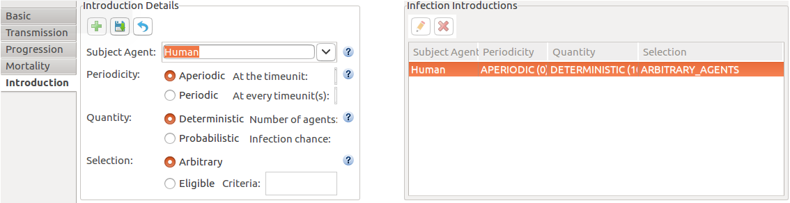
The introduction tab on the properties view specifies which, when and how many elements will be contaminated:

Subject Agent: the agent that will be subjected to the introduction.

Periodicity: when the disease introduction will happen.

Quantity: how many agents will be infected.

Selection: which agents will be infected.

Fig. 37 shows the box that represents the properties view to edit the disease introduction.

More than one agent can be subject to the same disease as shown in Fig. 38.