|
Eduardo S. L. Gastal eslgastal@inf.ufrgs.br |
and |
Manuel M. Oliveira oliveira@inf.ufrgs.br |
For up-to-date information refer to our Project Website:
http://inf.ufrgs.br/~eslgastal/NonUniformFiltering
Computer Graphics Forum.
Volume 34 (2015), Number 2, Proceedings of Eurographics 2015, pp. 81-93.
These are the supplementary materials for our paper presented at Eurographics 2015. If you wish to run the following examples in your machine, you must download our source code package from this link, then install SciPy, the julia language, and the IJulia notebooks. Please see the README.txt file in the source package for instructions on how to do this. To run the examples open the Supplementary.ipynb notebook using IJulia, otherwise open the static Supplementary.html file to see only the results in your browser of choice.
Table of Contents
- 1D Filtering Examples
- Edge-Aware Detail Manipulation Examples (Fig. 1 of our paper)
- Localized Editing Examples (Fig. 9 of our paper)
- Data-aware Interpolation (Fig. 10 of our paper)
- Non-Local Means Noise Reduction using Non-Uniform Filtering (Fig. 11 of our paper)
- Photograph Stylization (Fig. 12 of our paper)
- Video Filtering
# Load our code. This may take a few seconds to
# initialize the julia and scipy packages.
include("src/main.jl");
1D Filtering Examples
Impulse Response Accuracy (Fig. 5 of our paper)
The following code generates the plots from Fig. 5 of our paper. These plots show that our results are numerically accurate and visually indistinguishable from ground-truth, with PSNR consistently above 250 dB (note that a PSNR above 40 dB is already considered indistinguishable visual difference in image processing applications). Note that our mathematical formulation is exact, and our result differs from the ground-truth only due to the finite precision inherent to floating-point arithmetic.
include("src/Fig_5_impulse_response.jl")


Noisy Signal Band-pass Filtering (Fig. 6 of our paper)
The following code generates the plots from Fig. 6 of our paper. These plots illustrate the accuracy of our approach in filtering general non-impulse signals. The noisy non-uniformly sampled sinusoid in (a) is filtered by the band-pass Butterworth filter from Fig. 5 (previous section) using our approach. The filtered samples are shown in (b), superimposed on the original noiseless signal (in blue).
include("src/Fig_6_noisy_sinusoid.jl")


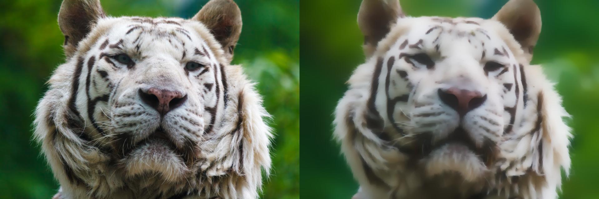
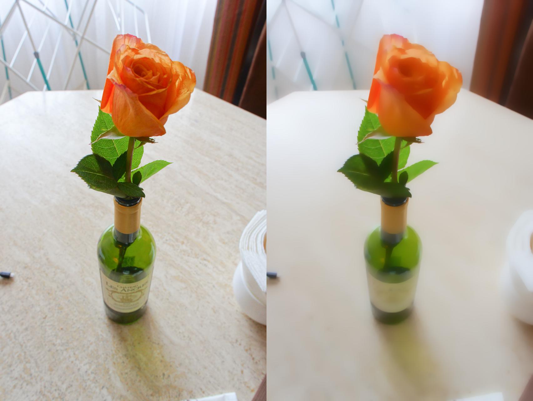
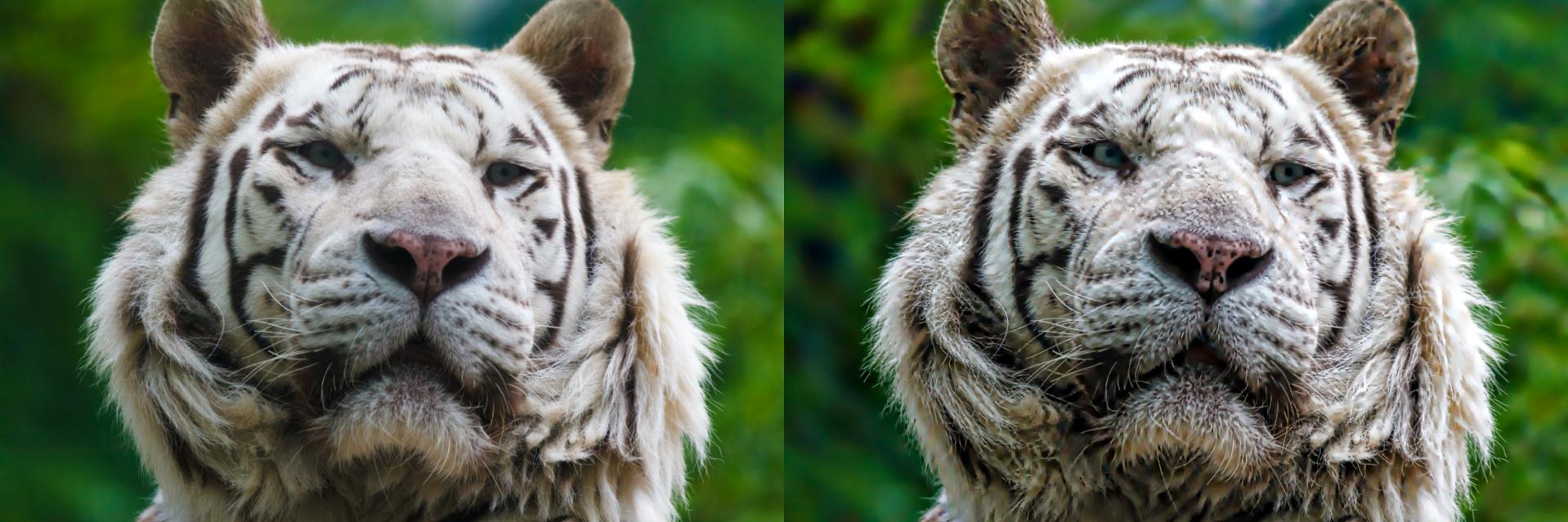
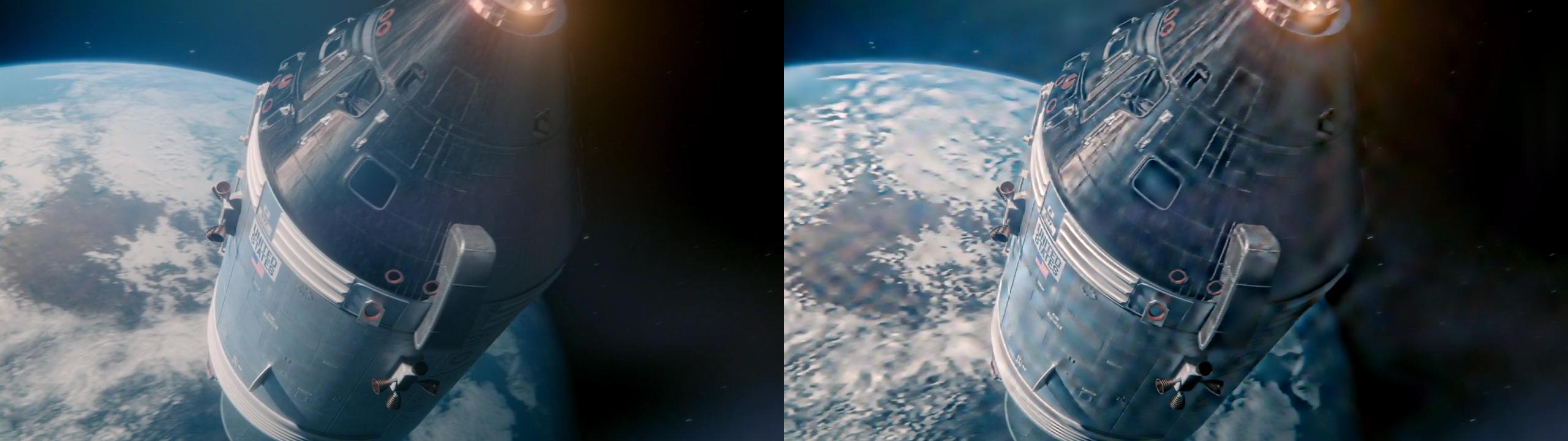
Edge-Aware Detail Manipulation Examples (Fig. 1 of our paper)
The following code generates the images from Fig. 1 of our paper. For these examples, non-uniform sampling positions are computed using an edge-aware transform. Thus, the resulting filters preserve the image structure and do not introduce visual artifacts such as halos around objects.
The filtering effects for these images have been exaggerated for illustrative purposes. The parameters for the filters can be controled in the function calls. σ_s and σ_r are parameters of the edge-aware filter. σ_s controls the imagespace size of the filter kernel, and σ_r controls its range size (i.e., how strongly edges affect the resulting filter). We refer the reader to [GO11] for further details.
Supplementary.ipynb, please note that filtered images are saved to disk in the filtered_images folder of the working directory.
References:
[GO11] Eduardo S. L. Gastal and Manuel M. Oliveira. "Domain Transform for Edge-Aware Image and Video Processing". ACM Transactions on Graphics. Volume 30 (2011), Number 4, Proceedings of SIGGRAPH 2011, Article 69.Website: http://inf.ufrgs.br/~eslgastal/DomainTransform
include("src/Fig_1_edge_aware_filters.jl")

# Add the filesystem path of an image file to this list and
# it will be used for filtering in the following examples.
filenames = [
    "images/white-tiger-head-pdp-94418.jpg",
    "images/DSC01252.jpg",
    "images/DSC02190.jpg",
    "images/black-rhinoceros-pdp-8661.jpg",
    "images/video_still.png",
    "images/flower4.png"];
Low-pass Gaussian filter
The low-pass edge-aware Gaussian filter smoothes small variations in the image while preserving large-scale features. It is a good filter for stylization or removing small variations in skin color in portraits photographs. The filtering effects for these images have been exaggerated for illustrative purposes — parameters should be adjusted for specific applications.
Fig_1_low_pass_gaussian(filenames, σ_s=50.0, σ_r=0.2)


Modified Laplacian of Gaussian
The modified band-stop Laplacian of Gaussian negates medium frequencies in the image, creating a stylized look for the scene.
Fig_1_modified_LoG(filenames, σ_s=50.0, σ_r=0.05)


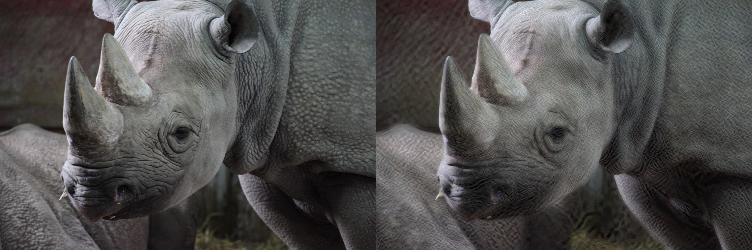


High-pass Enhancer (Butterworth)
The high-pass enhancer based on the Butterworth filter highlights fine details in the image, such as the tiger's whiskers, the flowers' petals, the rhinoceros' skin, and the statue's stone texture.
Fig_1_high_pass_enhancer(filenames, σ_s=50.0, σ_r=0.5)


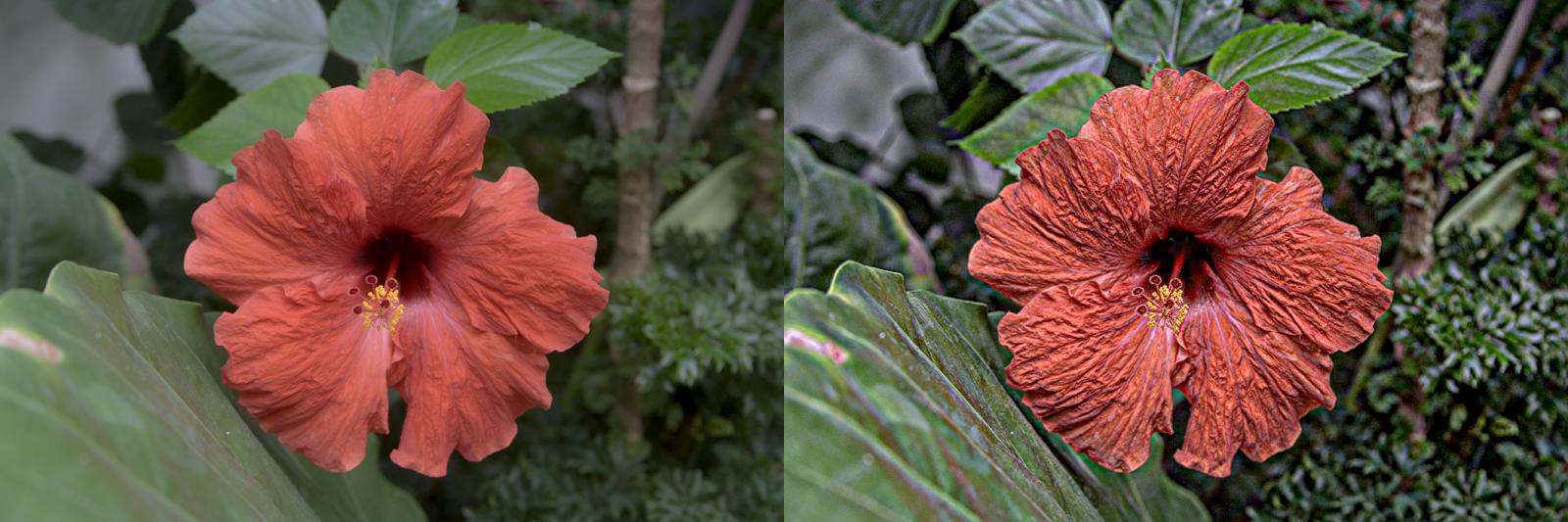
Band-pass Enhancer (Butterworth)
The band-pass Butterworth enhancer improves local contrast by boosting medium-scale details in the image. For these images, an edge-aware low-pass post-filter was applied to obtain the final result. See our paper for details.
Fig_1_band_pass_enhancer(filenames, σ_s=200.0, σ_r=0.2)


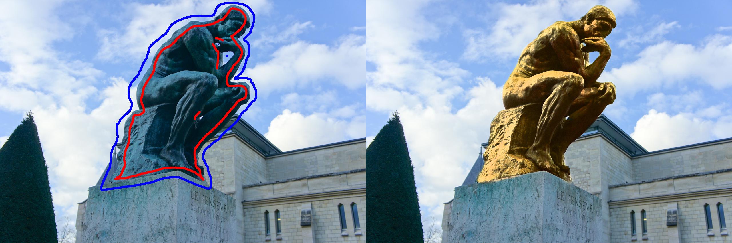
Localized Editing Examples (Fig. 9 of our paper)
The following code generates Fig. 9 of our paper. For this example, our non-uniform edge-aware low-pass Gaussian was used to locally change the color of the statue. On the left image, color scribbles define two regions of interest. For each region, we generate an influence map using edge-aware filtering. These influence maps are used to defined a soft segmentation mask, which is used to selectively change the color of the statue.
include("src/Fig_9_localized_editing.jl")
Data-aware Interpolation (Fig. 10 of our paper)
The following code generates Fig. 10 of our paper. This figure illustrates the use of our filters for sparse data interpolation. Our non-uniform filter propagates the color of a small set of pixels, shown in the Bottom-Left quadrant, to the whole image. This generates the full-color image shown in the Bottom-Right quadrant. The non-uniform domain is defined by the domain transform [GO11] computed from the lightness image in the Top-Right quadrant. The original image is shown in the Top-Left quadrant. Please refer to our paper for details.
include("src/Fig_10_data_aware_interpolation.jl")
Non-Local Means Noise Reduction using Non-Uniform Filtering (Fig. 11 of our paper)
The following code generates Fig. 11 of our paper. This figure illustrates the use of our formulation for denoising. The noisy photograph on the Top-Left quadrant is denoised using our non-uniform filters, generating the image on the Top-Right.
By grouping pixels based on high-dimensional neighborhoods, we can define a fast and simple denoising algorithm. We cluster pixels from the noisy photograph based on their proximity on the high-dimensional non-local means space. For this example, we generate 30 clusters using k-means, which are color-coded in the Bottom-Left quadrant for visualization. The pixels belonging to a single cluster define a non-uniformly sampled signal in the imagespace.
We apply a non-uniform low-pass filter only to the pixels belonging to the same clusters, averaging-out the zero-mean noise. Using our formulation, for an image with N pixels, filtering together only pixels belonging to the same clusters is done in O(N) time for all clusters. Please refer to our paper for details.
include("src/Fig_11_denoising.jl")

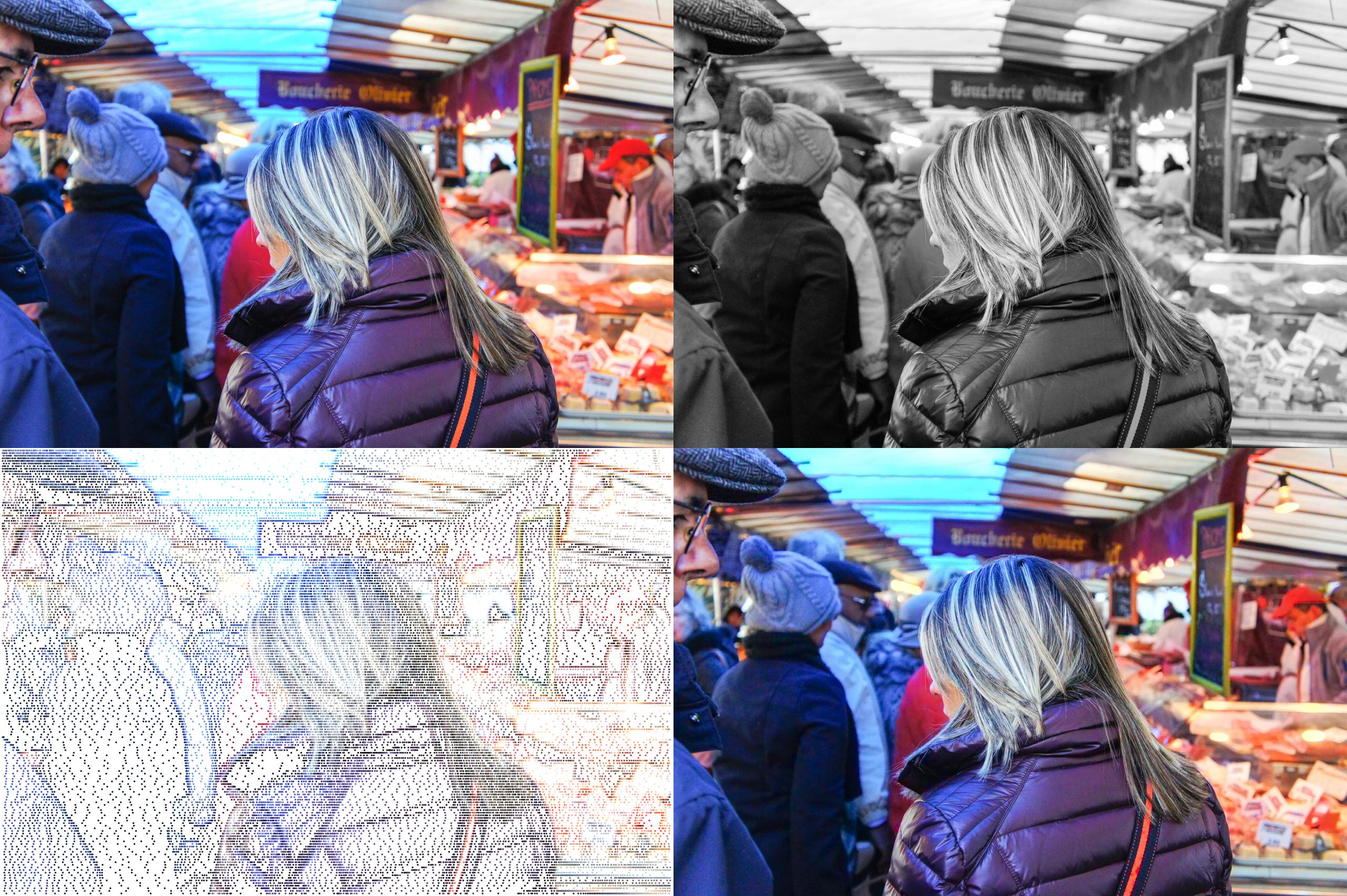
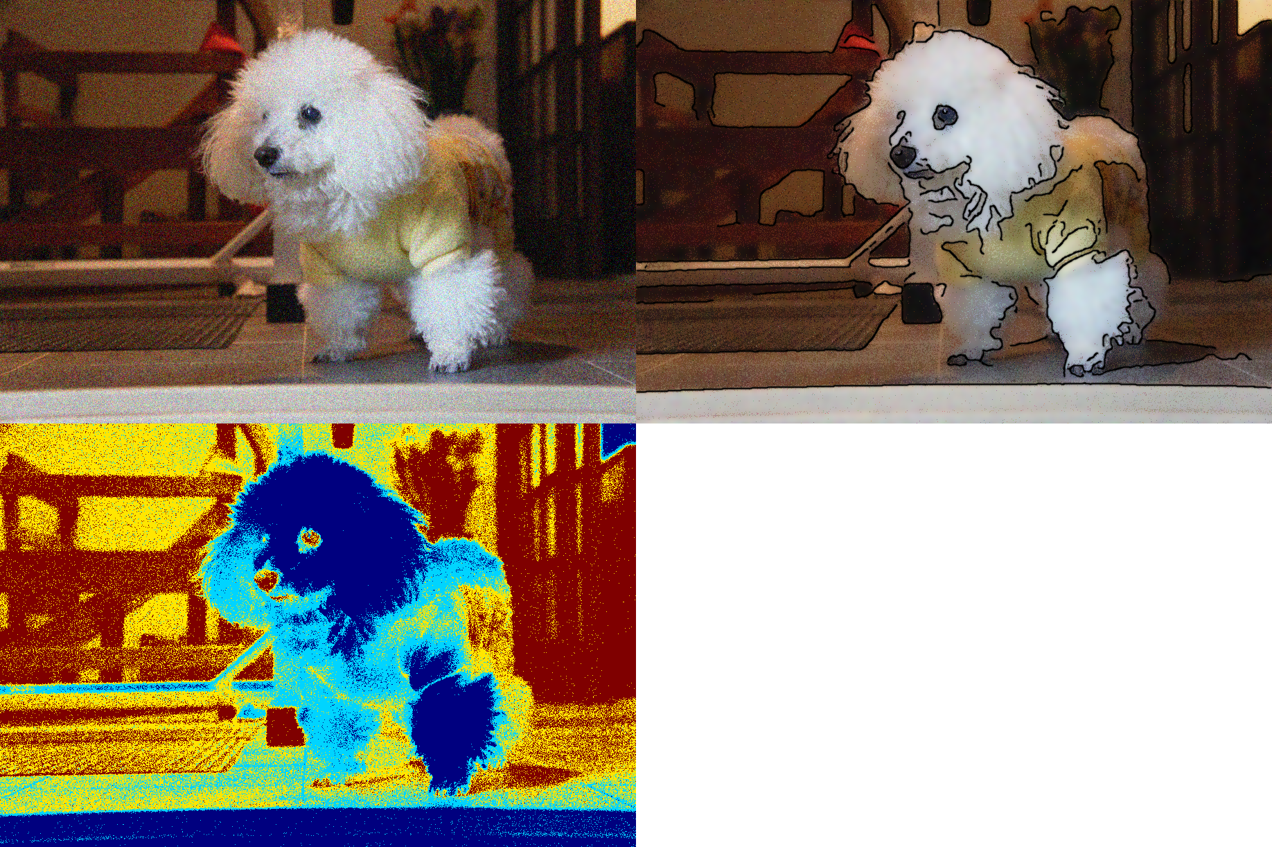
Photograph Stylization (Fig. 12 of our paper)
The following code generates Fig. 12 of our paper. This image illustrates how the same idea behind the denoising algorithm above can be used for stylization. In the Bottom-Left quadrant, we cluster pixels based only on their RGB-proximity. Filtering only pixels belonging to the same clusters with a non-uniform low-pass filter, and then superimposing edges computed using the Canny algorithm, one obtains a soft cartoon-like look, shown in the Top-Right quadrant.
include("src/Fig_12_stylization.jl")
Video Filtering
The code below applies our high-pass Butterworth enhancer filter to an HD video sequence. Note that the filtering result is temporally stable, which is true for all of our filters. The filtering result will always be temporally coherent if the non-uniform sampling scheme is temporally coherent. This example uses the domain transform which has been shown to produce stable filters [GO11].
The filtered video below contains a small amount of flickering in low-contrast regions due to the amplification of compression noise — ie, our source video has some high-frequency compression artifacts (blocking) which are also amplified together with high-frequency details.
You can open the videos by clicking on the local file links. The side-by-side video comparing the original and filtered video sequence is embeded in the HTML file. If you are using a modern browser, just hit play.
input_filename  = "videos/sample.ogv"
filtered_filename = "videos/filtered.webm"
sidebyside_filename = "videos/sidebyside.webm"

display("text/html", ipdisplay.FileLink(input_filename))
display("text/html", ipdisplay.FileLink(filtered_filename))
display("text/html", ipdisplay.FileLink(sidebyside_filename))
ipdisplay.HTML("""<center><video controls src="$sidebyside_filename" width="100%"/></center>""")
# Uncomment the following to lines to re-filter and re-encode
# the videos. This may take some time since our julia code is
# far from optimized. A better julia or even C++ implementation
# of our filters could process a video in real-time due to the
# linear O(N)-time performance of our formulation.

#include("src/video_filtering.jl")
#video_high_pass_enhancement(input_filename=input_filename)
#video_encode(filtered_filename=filtered_filename, sidebyside_filename=sidebyside_filename)