Creating the Traffic Signal Control simulation
This tutorial will show how to create the Traffic Signal Control to help understand the ABStractme tool features.
First create a new project and a new diagram, detailed instructions on the link: Creating the first project.
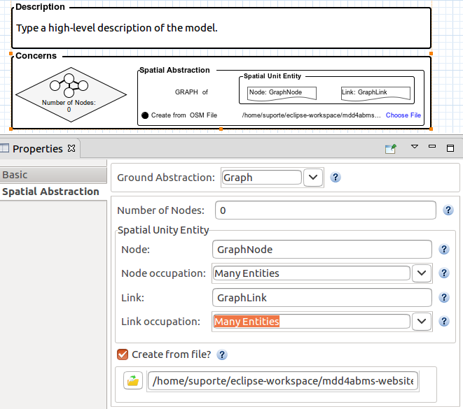
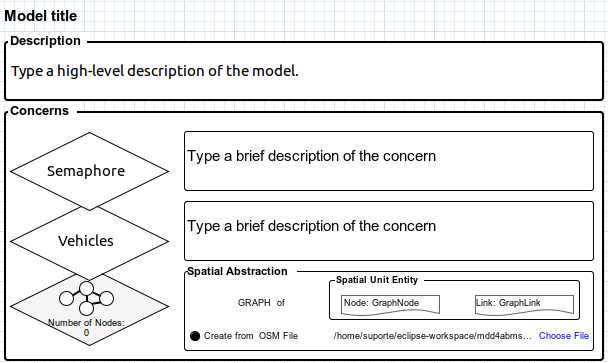
Open the diagram created, click on the overview box. At the properties view, select the "Spatial Abstraction" tab and change the "Ground Abstraction" combo box to "Graph". Mark the "Create from file?" field. A file to set the location of the graph nodes is needed. The file is available to download on the link below.
After downloading the file click on the folder button, on the opened window change the file type to search to "OSM File" and select the downloaded file.
The resulting properties view will look like Fig. 1.
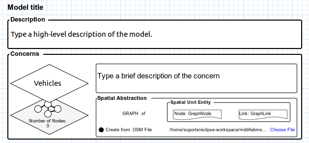
Now select the concern line on the palette and click on the overview rectangle.
A concern will be added to the overview along with its corresponding tab.
Select the concern diamond, on the properties view, set the name to "Vehicles".
The resulting overview will look like Fig. 2.
Click twice on the vehicle diamond. Select the concern tab that appeared, a new window will appear with the concern diagram.
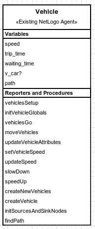
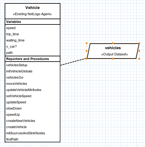
Now add a vehicle agent to the concern, this time it will be an existing NetLogo agent. A file to set this agent is necessary. The file is available to download on the link below.
After downloading the file, select the agent to add, by clicking on the External > "Existing NetLogo Agent" line on the palette and clicking anywhere on the concern diagram.
A window to select the downloaded file will appear. After selecting the file, the resulting agent box will look like Fig. 3.
Now add a graphic to monitor the number of vehicles that are not moving after every 45 time units, to see if there is a traffic jam.
To add the graphic, select one to add, by clicking on the Output > "Output Dataset" line on the palette and clicking anywhere on the diagram.
You can select the box created. On the properties view that appeared, focus on the left column.
You can choose a name to give to the graphic on the "Name" field, "vehicles" for example. Inside the output rectangle, click on the "+" button.
On the "Name" field, choose a name to identify the line to be added to the graphic. Let's call the line "stopped".
Also, choose the entity related to the defined line. On the "Entity" field select the agent created previously.
On the "Criterion" field select "Eligible" and set the field to "speed = 0".
On the "Periodicity" field set the number of time units to 45.
Leave everything else unchanged.
Click on the floppy disc button to save the changes.
If you select the line created on the right column of the properties view and click on the pencil button, the resulting "Output" properties will look like Fig. 4.
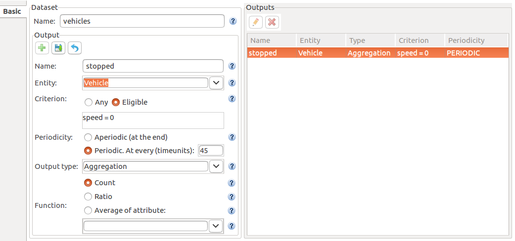
Fig. 5 shows what the entire vehicle diagram will look like after the changes made in this tutorial.
Now go back to the overview window that is the tab at the left of the concern tab. After returning to the overview window, close the vehicles concern tab.
Now select the concern line on the palette and click on the overview rectangle.
A concern will be added to the overview along with its corresponding tab.
Select the concern diamond, on the properties view, set the name to "Semaphore".
The resulting overview will look like Fig. 6.
Click twice on the semaphore diamond. A new window will appear with the concern diagram.
Now add an agent to the concern. Select an agent to add, by clicking on the agent line on the palette and clicking anywhere on the concern diagram.
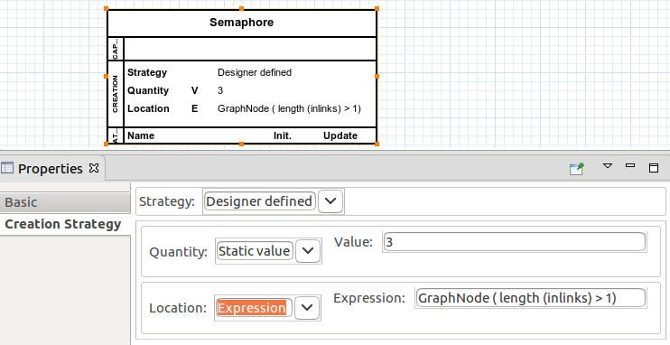
The agent box will appear on the diagram. Select the box. On the "Basic" properties view, you can name the agent, in our case, its name will be "Semaphore".
Change to the "Creation Strategy" tab, change the field "Strategy" to "Designer Defined", other fields will appear.
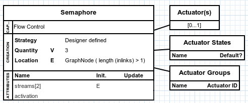
On the line that starts with "Quantity", set the "Value" field to 3 so that three semaphores will be part of the simulation.
On the line that starts with "Location", set the "Expression" field to "GraphNode ( length (inlinks) > 1 )".
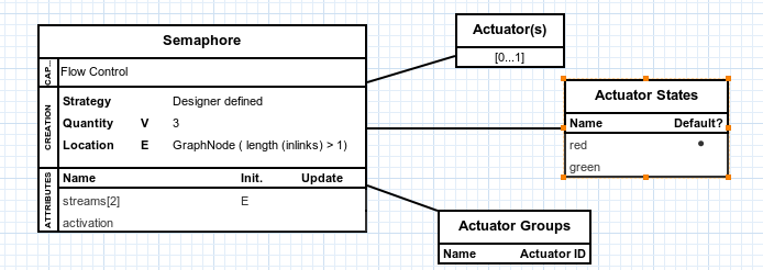
The resulting agent and properties will look like Fig. 7.
Now add the flow control capability to the agent to set up two plans for the semaphores.
Select the capability to add, by clicking on the Flow Control > "Flow Control Capability" line on the palette and clicking on the agent box.
Three new boxes will be added to the diagram, notice that they are connected to the agent.
The resulting agent box will look like Fig. 8.
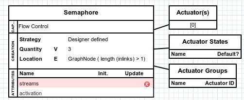
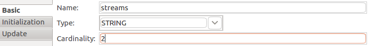
The agent received two new attributes, let's focus on stream attribute for now.
Select the stream attribute, on the properties view that appeared, "Cardinality" field, set the value to 2.
The resulting properties view will look like Fig. 9.
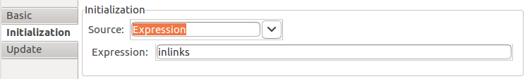
Change to the "Initialization" tab. Change the "Source" field to "Expression".
On the new line that appeared below, set the "Expression" field to "inlinks".
The resulting properties view will look like Fig. 10.
After the changes, the resulting agent box will look like Fig. 11.
Now add actuator states to the Actuator States box.
Select an actuator state to add, by clicking on the Flow Control > "Actuator State" line on the palette and clicking on the actuator states box.
A new line will be added to the box, select the line.
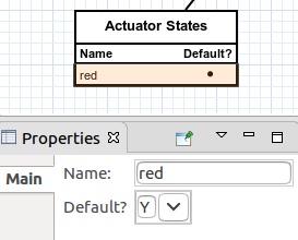
On the properties view that appeared, set the actuator state name to "red" and on the "Default?" field select "Y".
The resulting properties view will look like Fig. 12.
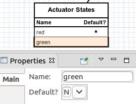
Add another actuator state by repeating the steps above, this time the name will be "green" and the "Default?" field will be "N".
The resulting properties view will look like Fig. 13.
After the changes, the resulting agent box will look like Fig. 14.
Now add the state machine to the agent.
Select a decision capability to add, by clicking on the Decisions > "State Machine" line on the palette and clicking on the agent box.
A new box will be added to the diagram, notice that it is connected to the agent.
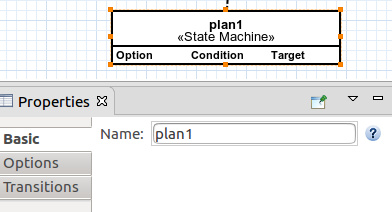
Select the created box. On the properties view that appeared, set the state machine name to "plan1".
The resulting box and properties view will look like Fig. 15.
Now connect the state machine to the flow control(actuators and actuator states).
Select a decision option to add, by clicking on the Decisions > "Decision Option" line on the palette and clicking on the state machine box first and then clicking on the actuator(s) box.
Select another decision option to add, by clicking on the Decisions > "Decision Option" line on the palette and clicking on the state machine box first and then clicking on the actuator states box.
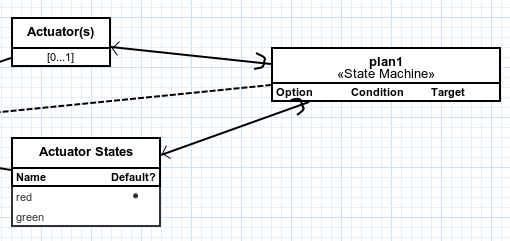
The resulting state machine box will look like Fig. 16.
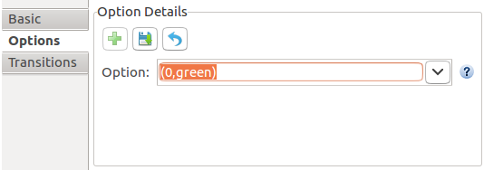
Click on the state machine box and change to the "Options" tab. Click on the "+" button to add an option to the state machine.
On the field "Option" select "(0,green)".
The resulting "Options" tab will look like Fig. 17.
Click on the floppy disc button to save the changes.
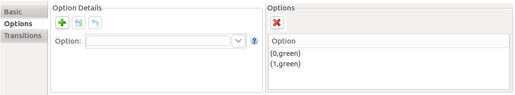
Click on the "+" button again.
On the field "Option" select "(1,green)".
Click on the floppy disc button to save the changes.
The resulting "Options" tab will look like Fig. 18.
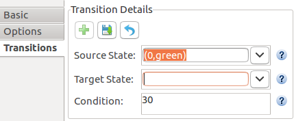
Change to the "Transitions" tab. Click on the "+" button to add a transition to the state machine.
On the field "Source State" select the "(0,green)" option.
On the field "Target State" leave the field empty.
On the field "Condition" set the value to 30.
The resulting "Transitions" tab will look like Fig. 19.
Click on the floppy disc button to save the changes.
Click on the "+" button to add another transition to the state machine.
On the field "Source State" select the "(1,green)" option.
On the field "Target State" select the "(0,green)" option.
On the field "Condition" set the value to 15.
Click on the floppy disc button to save the changes.
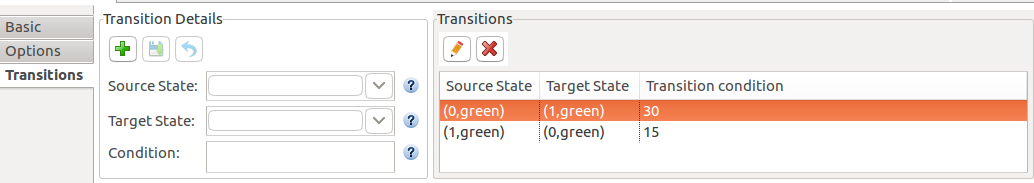
Select the first line created on the right column of the properties view(the one with the blank target state) and click on the pencil button.
On the field "Target State" select the "(1,green)" option.
Click on the floppy disc button to save the changes.
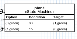
The resulting "Transitions" tab will look like Fig. 20.
The resulting state machine box will look like Fig. 21.
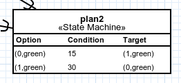
Create another state machine by repeating the steps above, its name will be "plan2" and on the transitions properties tab, the field "Condition" will be set in the opposite order, first 15 and then 30, as shown in Fig. 22.
Now add the learning capability to the agent.
Select a decision capability to add, by clicking on the Decisions > "Learning" line on the palette and clicking on the agent box.
A new box will be added to the diagram, notice that it is connected to the agent.
The resulting agent box will look like Fig. 23.
Now connect the learning capability to the state machines created previously.
Select a decision option to add, by clicking on the Decisions > "Decision Option" line on the palette and clicking on the learning capability box first and then clicking on the "plan1" state machine box.
Select another decision option to add, by clicking on the Decisions > "Decision Option" line on the palette and clicking on the learning capability box first and then clicking on the "plan2" state machine box.
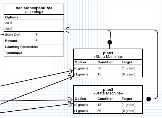
The resulting learning capability box will look like Fig. 24.
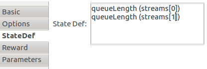
Click on the learning capability box and change to the "StateDef" tab.
Set the "State Def" field to "queueLength (streams[0])" in the first line and "queueLength (streams[1])" in the second line.
The resulting "StateDef" tab will look like Fig. 25.
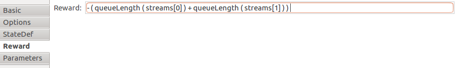
Change to the "Reward" tab.
Set the "Reward" field to "- ( queueLength ( streams[0] ) + queueLength ( streams[1] ) ) ".
The resulting "Reward" tab will look like Fig. 26.
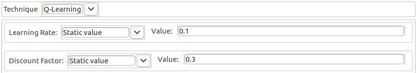
Change to the "Parameters" tab.
On the field "Technique" select "Q-Learning", other fields will appear:
On the field "Learning Rate" select "Static Value" and set the value to 0.1.
On the field "Discount Factor" select "Static Value" and set the value to 0.3.
The resulting "Parameters" tab will look like Fig. 27.
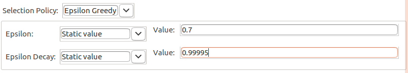
On the field "Selection Policy" select "Epsilon Greedy", other fields will appear:
On the field "Epsilon" select "Static Value" and set the value to 0.7.
On the field "Epsilon Decay" select "Static Value" and set the value to 0.99995.
The resulting "Parameters" tab will look like Fig. 28.
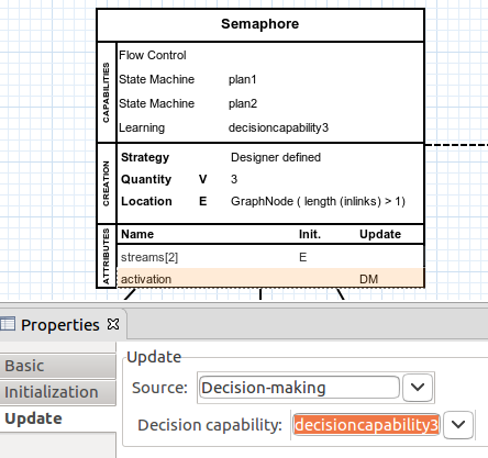
Now select the activation attribute on the agent.
On the properties view change to the "Update" tab.
On the "Source" field select "Decision-Making", on the line that appeared below, field "Decision Capability", select the learning capability created previously.
The resulting "Update" tab will look like Fig. 29.
Now select each state machine, "Transition" properties tab, and change the transitions that have (1,green) as source state.
Select the corresponding line on the right column of the properties view(the one with the (1,green) as source state) and click on the pencil button.
On the field "Target State" select the "Terminal" option.
Click on the floppy disc button to save the changes.
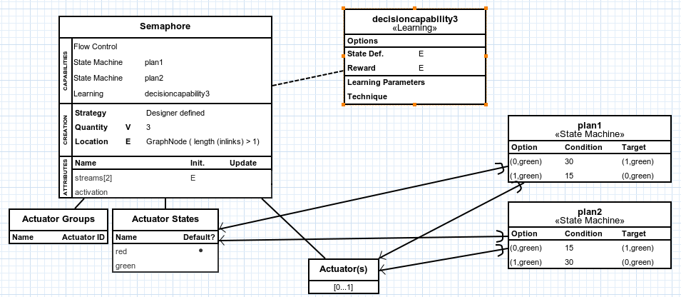
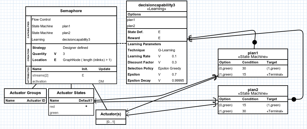
Fig. 30 shows what the entire concern diagram will look like after the changes made in this tutorial.
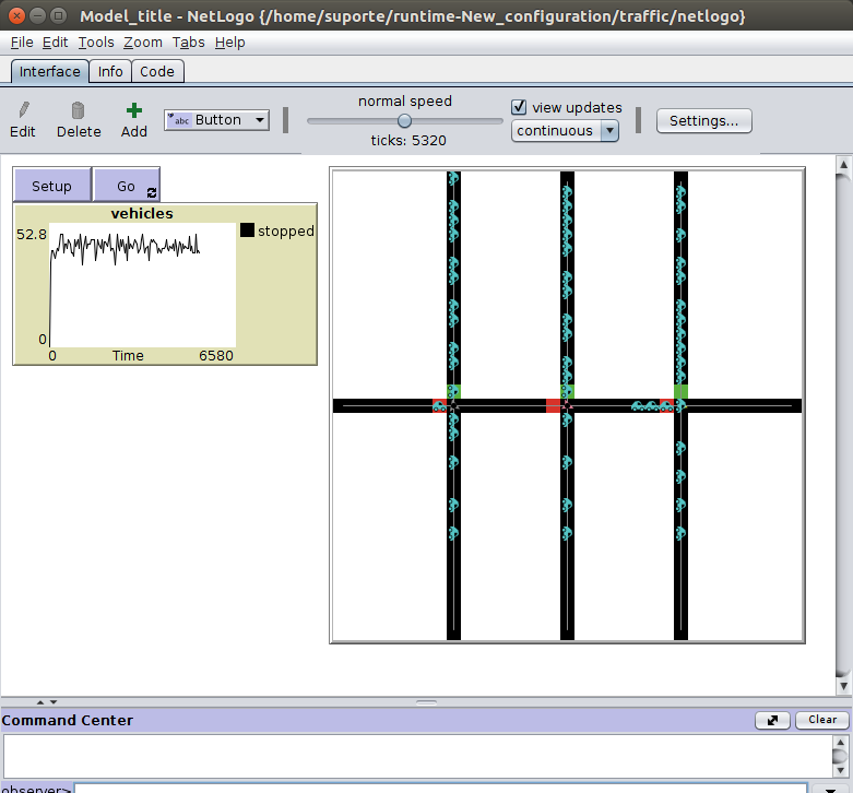
Now export and run the simulation on NetLogo, detailed instructions on the link: Exporting the Project to NetLogo.
The simulation will look like Fig. 31.
The complete project created on this tutorial is available to download on the link below.