Quickstart Guide
Getting started
This tutorial serves as a quickstart guide to GEAP by introducing a basic example of performing a microarray analysis from the input source to the final results.
We tried to make it simple by omitting more specific cases and keeping the default parameters, but these steps still serve as a basis which may be adapted by the user for each particular example.
Before following the steps below, download and run GEAP on your computer.
Browsing GEO
The Gene Expression Omnibus (GEO) is the largest database for large-scale gene expression datasets and our primary source for microarray data. You can browse it using search terms to find the results of experimental studies according to your interests. However, to better understand GEO's search entries, some basic concepts must be taken into account.
GEO Basic Concepts
An experimental result is defined as a GEO Series (GSE) and identified by a code marked with the GSE prefix (e.g., GSE12345). It consists of a table of gene expression detection values and some experimental details concerning the study. Besides, if GEO curated the data, there's a correspondent GEO Dataset (GDS) entry to this GSE.
Each numeric column has its entry in a GSE table identified as a GEO Sample (GSM). The numeric values in a GSM represent the probe detection in an experimental sample.
There's an identifier column representing the probe names related to the detection values in both GSE and GSM. The probes used in a GSM are described by a GEO Platform (GPL), whose main content is a table that associates each probe to the gene transcripts and other attributes.
The table below summarizes the GEO accession types above, and you can find more details on the GEO Overview documentation page.
| Prefix | Full name | Description |
|---|---|---|
| GSE | GEO Series |
Describes the results for an experimental study. Contains a set of GSM entries concatenated into a single table* |
| GDS | GEO DataSet |
Curated information for a GSE used in GEO display and analysis tools. Every GDS has a correspondent GSE, but not every GSE has a GDS |
| GSM | GEO Sample |
Table of microarray detection values. Probe identifiers belong to a specific GPL |
| GPL | GEO Platform |
Table of descriptors related to a probe set. Associates each probe to one or more gene transcripts |

In most cases, you will be searching for a GSE to evaluate your own case study. In the next section, we're going to find a GSE as the input to our analysis.
Browsing a GSE
- Go to GEO Datasets and enter a search term;
-
(Optional) Apply some filters to restrict the results. They are located at the page's left sidebar.
We suggest applying the following filters:-
Seriesas the Entry Type to search only GSE entries -
Expression Profiling by Arrayas the Study Type to search only microarray experiments
-

Tips when browsing in GEO:
- You can include some advanced terms to restrict the search results – for example,
(Mus musculus[organism])will return only experiments that include mice as the organism model; - Sample replicates are crucial for statistical accuracy. Avoid GSEs lacking replicates (i.e., only one GSM per experimental condition);
- Be extra careful with unpublished results, since you can't compare your analyses with those performed by the author.
- If you find a suitable GSE, click on the title to view the accession details.
In this example, we'll be using GSE39009, a study involving the gene expression profile of Yin Yang 1 (YY1) knockout mice;

- Check the information regarding the study. It's advisable to read the published article (if available) to understand the experimental assays;
- Copy the GSE code to clipboard – or if you prefer, just memorize it – as you'll need it afterwards in GEAP.
In this example, the code isGSE39009

The GSE code is the simplest and most straightforward input that can be given to GEAP.
In the next step, we'll use this code to tell the program to download and process our GSE.
Pre-Analysis
Data Input
- Open GEAP;
- Click on the Start Analysis button;

- Click on the Series (GSE) button, since we're going to use a GSE as input;

Now we must provide input to the program. The program presents three methods of loading data inputs: Web Download, Local File and Library File. In this example, we will request the data set by providing the GSE code to GEAP and letting the program take care of downloading from the Web (hence, Web Download option).
- Paste the GSE code into the GSE Code: text box located inside the Web Download option;
- Check the Load Probe Information (GPL) check box, if not already checked. This option will include the series' GPL in the download queue;
- Check the RAW Data Analysis check box if you want to analyze data in the RAW format.
Regarding this option:- If unchecked, the program will download the preprocessed table with the author's parameters for statistical treatment;
- If checked, the program will download the source data in the raw format. Afterward, some additional steps will be needed to perform the statistical treatment – we'll cover them in the next part;
Note: Always check this option for dual-channel microarrays, as their preprocessed formats usually include log-ratios instead of array intensity values for each channel.
Working with dual-channels in the author's format (instead of the RAW) may give unexpected results. - Click on Load and wait for the program to collect info regarding the GSE. Make sure your internet connection is properly working;

- Confirm the name of the desired series and click on Yes, load it;
- Wait while the program downloads and inspects the dataset files. If you opted for the Raw Data Analysis option, some required dependencies will be automatically downloaded in this step;

Platform Selector
- After downloading and checking the inputs, the program will prompt a dialog box where you can select which data inputs should be loaded or not. Which files will appear depends on whether you checked the RAW Data Analysis option.
-
If Raw Data Analysis option remained unchecked:
There's no statistical treatment step. Click on the Load button and jump to the Session Overview section;
-
If Raw Data Analysis option was checked:
Click on the Load button and follow the next steps;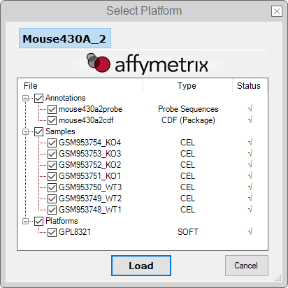
Raw Statistical Treatment
Microarray files in the RAW format must be processed beforehand to become an analyzable matrix. This step is called Statistical Treatment.
Every platform has its statistical treatment methods depending on the data format and manufacturer, and every method also has its parameters. The parameter preference over another is up to the user's expertise in statistics, but some fundamental concepts are common among these methods.
Some treatment concepts are more present, such as the Background Correction and Normalization, while others like Perfect-match correction and Summarization are more platform-specific. The table below has a brief description of them:
| Parameter | Usage | Applied in |
|---|---|---|
| Background correction | Corrects errors related to probe signal absorbance and background noise (e.g., due to light scattering) | All data sources including a background matrix |
| Normalization | Adjusts the detection values to keep all samples in the same scale (e.g., correcting level errors) | All data sources |
| Perfect-match correction | Corrects the probe signals based on the distinction between probes that perfectly match their transcripts and probes with a single pair mismatch that still emit a hybridization signal | Affymetrix microarrays |
| Summarization | Combines the probe detection values into one representative value to the transcript levels | Affymetrix microarrays |
In the current example, we use the Expresso method for Affymetrix microarrays, which includes all parameters above.
For more treatment methods supported by GEAP, see the Reference Guide.
- We'll keep the default parameters for this example. Click on the Start Treatment button and wait for a while. After processing, the program will lead us to the Session Overview;

Session Overview
In GEAP, a Session represents a workspace for the processed microarray data. You can use this panel to access all collected and processed information from pre-analysis. For example, this includes details about the experimental procedures in the GSE, the metadata describing the GSM and GPL, or even machine specifications contained in some RAW data sources. You can also save the current Session as a "Project" and access it later.
- This panel is the start point to the next analyses in this example:
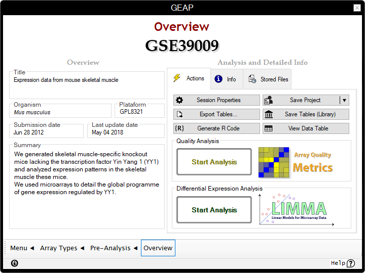
Quality Analysis (Optional)
Even the most robust statistical treatment cannot cure a poor quality array. Fortunately, we can apply some advanced analytical techniques to measure the data quality itself, thereby discarding samples that may introduce bias during other analyses.
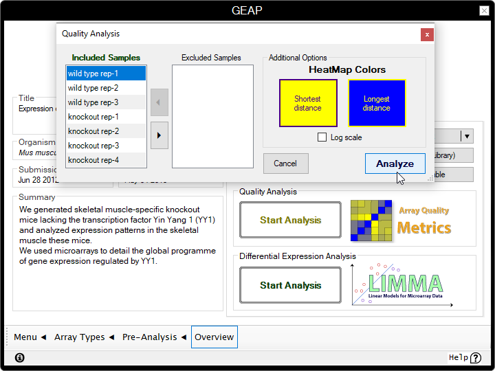
In this step, we're going to use GEAP to evaluate the array quality of the processed data.
- Inside the Quality Analysis box, click on the Start Analysis button;
- We'll keep the default parameters for this example, but you can use the leftmost panels to include/exclude samples from the analysis in another occasion;
- Click on the Analyze button and wait until the program finish the analysis. This process may take a few minutes.
The quality evaluation used by the program can be divided into four sections, whereas the first three sections are dedicated to find outliers. The purpose of each section is listed below:
- Section 1: Finds the outliers based on the sum of distances between one sample and all other samples;
- Section 2: Finds the outliers based on the distribution of probe detection values in one sample accross all other samples;
- Section 3: Finds the outliers based on deviations of probe detection values in an individual sample;
- Section 4: Generates a density plot to illustrate deviations accross all detection values.
More details can be found in the Reference Guide.
-
You'll be redirected to another page showing an overview of the quality analysis results.
The left panel shows the validation status for each sample, whereas the right tabs display some representative plots for each section.
In the absence of outliers in a sample, the status will appear asOK, which means that there aren't any outliers in the current example.
GSE39009 (current example): No outliers
In other cases, however, samples containing outliers will appear marked with the section number from where the outlier was encountered. Outliers may also appear in multiple sections, suggesting a bad quality in most cases.
GSE2600 (another GSE): Outlier at Section 2 found in the last sample
- (Optional) Reading the sample list as "GSM" codes may be counterintuitive for most users. You can change way that the samples are displayed by right-clicking on the table and selecting the attribute to be shown for each sample from the "View As" menu.


- (Optional) You can view the full report or export the results in HTML format. The buttons at the bottom-left are self explanatory.
- Use the navigation bar located at the bottom of the Window to return to the Session Overview page (Overview ◀ button).
Differential Expression: Comparison
In this step, we will evaluate our case study's biological conditions to find which genes are differentially expressed.
- Inside the Differential Expression Analysis box, click on the Start Analysis button;

- In our example, we're using the
GSE39009, which has only two conditions (YY1 knockout mice and wild type mice), so we'll perform a simple Experiment vs. Control comparison.
Click on the Comparison Between Two Groups (Experiment VS Control) button;

In the following page, you are presented with three boxes:
the avaiable Samples on the center,
the Experiment group at left,
and the Control group at right.
- (Optional) You may want to change the way that the samples are displayed by right-clicking on the table and selecting the attribute to be shown for each sample from the "View As" menu.

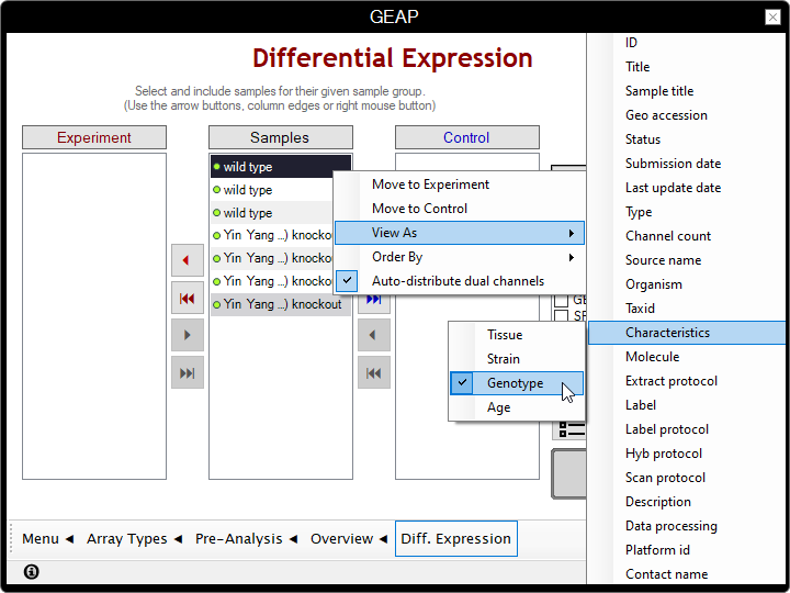
- Distribute the samples to the correspondent boxes according to their respective condition.
In this example, we're moving the knockouts to Experiment and wild types to Control;
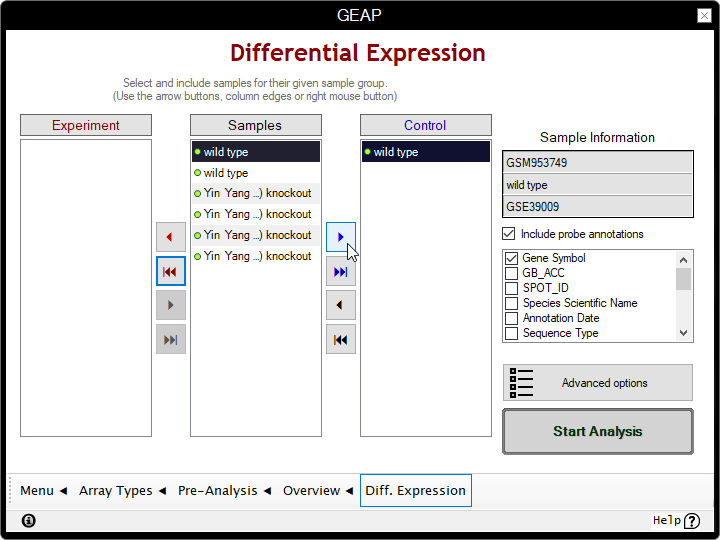
- If platform columns are present, check which columns you'll want to append to the results. Gene Symbols are checked by default.
- Click on Start Analysis and wait for the program to finish our analysis.

Differential Expression: Results
Viewing the results
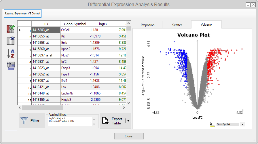
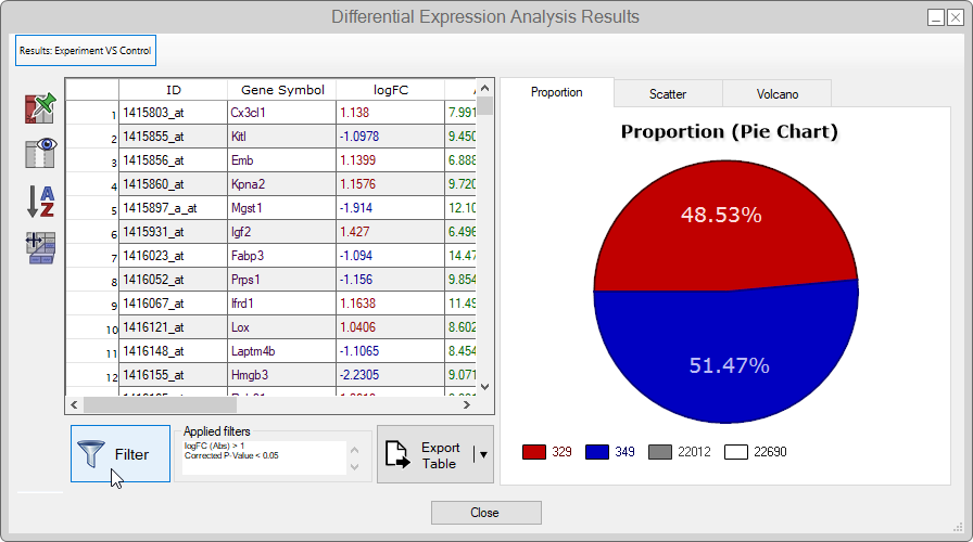
- Upon finishing the analysis, we'll be redirected to a page showing a summary table with the lowest and highest logFC values, as well as a pie chart displaying the proportion between over and under-expressed genes.
- Clicking the Full Table button will display a dialog window with the full results table.

Diff. Expression page > Advanced Options
Diff. Expression page > Advanced Options.
However, remember that this situation may also denote low statistical significance or bad array quality.
More than just displaying the full table, this menu also provides features to organize and filter the table
contents.
You can use the dynamics plots to explore the results by clicking on the data points,
which will propagate the table entries' selection.
Finally, you can Export Table as a text file or save the results as a project for the current Session
(closing this dialog, in the Actions tab > Register comparison data).
For more details about the features in this menu, see the Reference Guide.
Filtering the results (Optional)
- To apply your own custom filters to the table, click on the Filter button;
- Since this study is about Yin Yang 1 KO (YY1), let's find the entries containing yy1.
To this end, we must create a custom filter with the following parameters:-
Column:
Gene Symbol -
Condition:
Contains -
Value:
yy1 - Absolute unchecked (ignore case)
-
Column:


This way, the filter will find all rows where the "Gene Symbol" column "Contains" the "yy1" value (case insensitive).
By applying the filter, you'll see two filtered rows for the YY1 gene ‐ in other words, there are two correspondent probes to the same gene. Corroborating to the study, both probes present a significant and under-expressed logFC because the YY1 gene is "knocked out".

This way, you can establish your parameters of significance and apply custom filters to find your own targets based on your needs.
What to do next?
The differentially expressed genes could be used as input, for example, in other bioinformatic tools like STRING to create biological networks. If you're interessed in the biological context of your significant genes, GEAP also provides a feature to analyze Gene Ontologies, which we'll to cover in a future tutorial.